🗣️ Speech Analysis Using Parselmouth
- 16 minsTutorial on using Parselmouth in Python to estimate Pitch and Formants
About the Dataset 🗃️
The dataset contains Vowels and consonants in the Hindi Language organised based on place and manner of articulation recorded in my voice.The dataset contains a total of 39 phonemes. 14 are Vowels and 25 are Consonants.
The Dataset contains 2 Folders Vowels & Plosives.
Each File is a wav file sampled at 44100KHz and a bit resolution of 16bits/sample. The wav files are named by finding the equivalent letter available on keyboard to some of the symbols. Hence to avoid confusion they are kept in different sub-divided folders.
- Vowels(14) are further subcategorized into folders on the basis of
- Primary(10)
- Short(5)
- Long(5)
- Secondary(4)
- Long(2)
- Dipthongs(2)
- Primary(10)
- Plosives(25) are divided on the basis of Place of coarticulation into:
- Velar(5)
- Labial(5)
- Apico-Dental(5)
- Retroflex(5)
- Palatal(5)
Note:This has been done to make nasal sound names in the folders distinguishable.
Importing Libraries
- Parselmouth is a Python library that provides a convenient interface for working with Praat, a popular software tool for phonetic analysis. With Parselmouth, you can automate and streamline your phonetics research in Python
# Importing Libraries
import parselmouth
import numpy as np
import matplotlib.pyplot as plt
import seaborn as sns

sns.set()  # Use seaborn's default style to make attractive graphs
plt.rcParams['figure.dpi'] = 100  # Show nicely large images in this notebook
Load Datafile
For in depth understanding of my approach, I would be demonstrating the vowel ‘aa’
Load an audio file
snd = parselmouth.Sound("/content/drive/MyDrive/Data/Vowels/Primary/Long/a_.wav")

# Defining Functions

# Function to draw a spectrogram
def draw_spectrogram(spectrogram, dynamic_range=70, title="Spectrogram"):
    X, Y = spectrogram.x_grid(), spectrogram.y_grid()
    sg_db = 10 * np.log10(spectrogram.values)
    plt.figure()
    plt.title(title)
    plt.pcolormesh(X, Y, sg_db, vmin=sg_db.max() - dynamic_range, cmap='afmhot')
    plt.ylim([spectrogram.ymin, spectrogram.ymax])
    plt.xlabel("Time [s]")
    plt.ylabel("Frequency [Hz]")

# Function to draw intensity values
def draw_intensity(intensity):
    plt.plot(intensity.xs(), intensity.values.T, linewidth=3, color='w')
    plt.plot(intensity.xs(), intensity.values.T, linewidth=1)
    plt.grid(False)
    plt.ylim(0)
    plt.ylabel("intensity [dB]")

# Function to draw Pitch Values
def draw_pitch(pitch):
    # Extract selected pitch contour, and
    # replace unvoiced samples by NaN to not plot
    pitch_values = pitch.selected_array['frequency']
    pitch_values[pitch_values == 0] = np.nan
    plt.plot(pitch.xs(), pitch_values, 'o', markersize=5, color='w')
    plt.plot(pitch.xs(), pitch_values, 'o', markersize=2)
    plt.grid(False)
    plt.ylim(0, pitch.ceiling)
    plt.ylabel("fundamental frequency [Hz]")
Estimate Pitch & Formants using Spectral Analysis
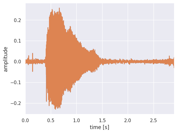
Plotting Signal
plt.figure()
plt.plot(snd.xs(), snd.values.T)
plt.xlim([snd.xmin, snd.xmax])
plt.xlabel("time [s]")
plt.ylabel("amplitude")
plt.show()
# or plt.savefig("sound.png"), or plt.savefig("sound.pdf")
Plotting Intensity & Spectrogram
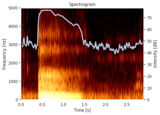
# Plotting Intensity Values on Spectrograms
intensity = snd.to_intensity()
spectrogram = snd.to_spectrogram()
plt.figure()
draw_spectrogram(spectrogram)
plt.twinx()
draw_intensity(intensity)
plt.xlim([snd.xmin, snd.xmax])
plt.show()
Plotting & Estimating Pitch
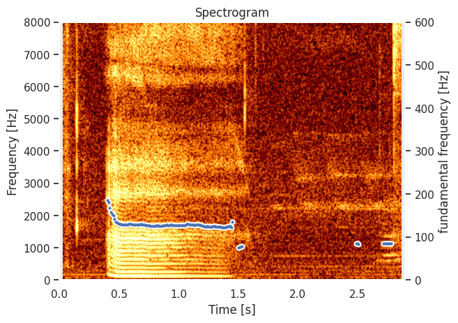
Estimate pitch
# Estimate pitch
pitch = snd.to_pitch()
pitch_values = pitch.selected_array['frequency']
pitch_times = pitch.xs()
average_pitch = sum(pitch_values) / len(pitch_values[pitch_values > 0])

# If desired, pre-emphasize the sound fragment before calculating the narrowband spectrogram
pre_emphasized_snd = snd.copy()
pre_emphasized_snd.pre_emphasize()
spectrogram = pre_emphasized_snd.to_spectrogram(window_length=0.03, maximum_frequency=8000)

plt.figure()
draw_spectrogram(spectrogram)
plt.twinx()
draw_pitch(pitch)
plt.xlim([snd.xmin, snd.xmax])
plt.show()
Plotting Formants
Maximum number of formants considered is 6 as it got better values. When considering lesser values, formants were estimated according to the overall trend.
# Compute the wideband spectrogram and estimate the pitch
wideband_spectrogram = snd.to_spectrogram(window_length=0.01, time_step=0.005)

wideband_segment = snd.extract_part(from_time=wideband_spectrogram.xmin, to_time=wideband_spectrogram.xmax, preserve_times=True)

# Estimate the first three formants for the wideband segment
wideband_formants = wideband_segment.to_formant_burg(max_number_of_formants=6)

# Extract times from the Pitch object for plotting the formants on the wideband spectrogram
pitch = wideband_segment.to_pitch()
formant_times = pitch.xs()

draw_spectrogram(wideband_spectrogram, title="Wide Band Spectrogram")

# Plot the formants on the wideband spectrogram
for i in range(3):
    formant_values = [
        wideband_formants.get_value_at_time(formant_number=i + 1, time=t)
        for t in formant_times
    ]
    plt.plot(formant_times, formant_values, color='w', linewidth=2, label=f'Formant {i + 1}')

plt.show()
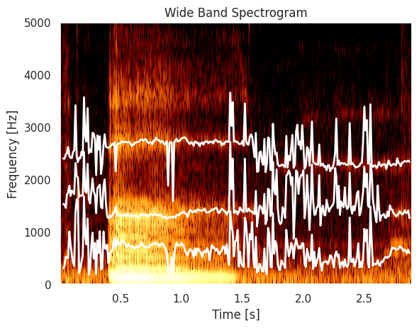
- We can see that the formants are not very clear from the image for the vowel.We would need to apply smoothing to the formants to get better approximate formants.
Plotting Smoothed Formants
# Function to apply smoothing to formant values
def smooth_formants(formant_values, window_size):
    smoothed_values = np.convolve(formant_values, np.ones(window_size) / window_size, mode='same')
    return smoothed_values

# Plot the formants on the wideband spectrogram
for i in range(3):
    formant_values = [wideband_formants.get_value_at_time(formant_number=i + 1, time=t) for t in formant_times]

    # Apply smoothing to formant values
    smoothed_formants = smooth_formants(formant_values, window_size=60)
    plt.plot(formant_times, smoothed_formants, color='b', linewidth=2, label=f'Formant {i + 1}')

plt.show()
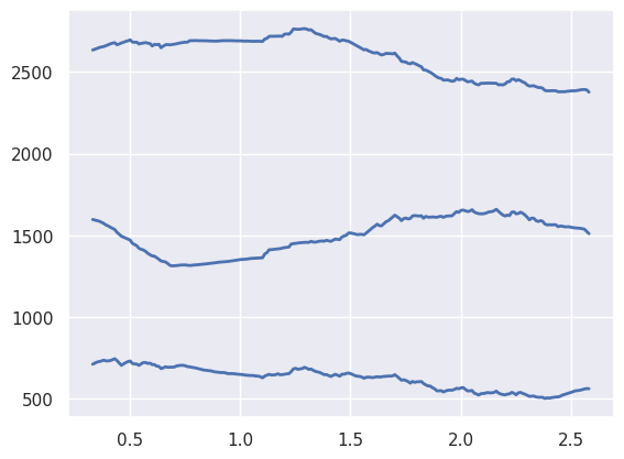
- In practice it is possible that we might only recieve upto 2 formants as the others are getting averaged out due to the other 2 being more dominant.
Estimate Pitch & Formants using Cepstral Analysis
Now we would try to estimate the pitch and Formants using the Cepstral Analysis.
- Since Praat doesn’t offer ceptstral analysis.We would require to do it manually.
# Importing Libraries
from scipy.signal.windows import hamming
import math
import numpy as np
from scipy.fft import fft, ifft
import scipy.io.wavfile as wav

## Windowing Signal

# Windowing using Hamming Function
w = hamming(math.floor(0.065 * snd.sampling_frequency), sym=False)  # Convert the window length to an integer


def create_overlapping_blocks(x, w, R=0.1):
    n = len(x)
    nw = len(w)
    step = math.floor(nw * (1 - R))
    nb = math.floor((n - nw) / step) + 1

    B = np.zeros((nb, nw))

    for i in range(nb):
        offset = i * step
        B[i, :] = w * x[offset:nw + offset]

    return B


# Call the function with 'snd1' and 'w'
B = create_overlapping_blocks(np.array(snd)[0], w)
print(B.shape)  # Print the shape of the resulting matrix


def compute_cepstrum(B):
    # Compute the FFT of the audio signal
    fft_result = fft(B)

    # Compute the logarithm of the absolute value of the FFT
    log_abs_fft = np.log(np.abs(fft_result))

    # Compute the inverse FFT (iFFT) of the result
    snd1 = np.real(ifft(log_abs_fft))
    return snd1


snd1 = compute_cepstrum(B[10])

## Plotting Cepstra

plt.plot(snd1)

## Estimating Pitch

pitch_quefrency = (300 + np.argmax(snd1[300:500])) / 44100
pitch_frequency = 1 / pitch_quefrency

pitch_frequency
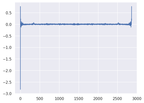 128.57142857142858
We can see the pitch values are matching for both the methods.Hence it cross verifies the result.
Estimating Formants
from scipy.signal import find_peaks

# Initialise the subplot function using number of rows and columns
figure, axis = plt.subplots(6, 2)
quefrencies = np.array(range(len(B[0]))) / 44100
frequencies = np.array(range(len(B[0]))) * 44100 / len(B[0])

for i in range(6):
    cepstrum = compute_cepstrum(B[i + 6])
    # Suppressing large values
    cepstrum[0] = 0
    cepstrum[1] = 0
    # Plotting cepstrum sequence
    axis[i, 0].plot(
        quefrencies[0:math.floor(len(quefrencies) / 2)],
        cepstrum[0:math.floor(len(cepstrum) / 2)],
        linewidth=0.5,
    )
    liftered_cepstrum = np.zeros(len(cepstrum))
    # Liftering the signal
    for j in range(80):
        liftered_cepstrum[j] = cepstrum[j]
    # Obtaining log compressed cepstrally smoothed spectrum
    cepstrally_smoothed_spectrum = fft(liftered_cepstrum)

    # Plotting log compressed cepstrally smooth spectrum
    axis[i, 1].plot(frequencies[0:150], cepstrally_smoothed_spectrum[0:150])
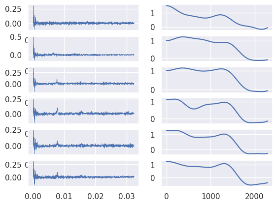
- We can see the formants from the 6 consecutive frames choosen at random.
Plotting Multiple Pitches
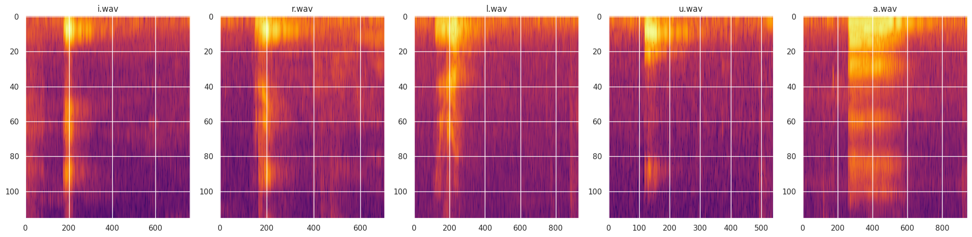
To make the pitches more visible and highlight them, we’ve applied the log to the spectrogram values to be able to differentiate between the pitch aspects of the different vowels
Spectrograms for Short Primary Vowels
import os
import parselmouth
import matplotlib.pyplot as plt
import numpy as np

# Directory containing your WAV files
dir = "/content/drive/MyDrive/Data/Vowels/Primary/Short/"
wav_files = [file for file in os.listdir(dir) if file.endswith(".wav")]

# Set the figure size
plt.figure(figsize=(20, 5))

# Create a row of subplots
num_plots = len(wav_files)
for i, wav_file in enumerate(wav_files):
    sound = parselmouth.Sound(dir + wav_file)
    spectrogram = sound.to_spectrogram()

    plt.subplot(1, num_plots, i + 1)

    # Adjust color mapping and dynamic range for better visibility
    plt.imshow(10 * np.log10(spectrogram.values), aspect='auto', cmap="inferno")  # Adjust cmap as needed
    plt.title(wav_file)

# Adjust the layout
plt.tight_layout()
plt.show()
Spectrograms for Long Primary Vowels
import os
import parselmouth
import matplotlib.pyplot as plt
import numpy as np

# Directory containing your WAV files
dir = "/content/drive/MyDrive/Data/Vowels/Primary/Long/"
wav_files = [file for file in os.listdir(dir) if file.endswith(".wav")]

# Set the figure size
plt.figure(figsize=(20, 5))

# Create a row of subplots
num_plots = len(wav_files)
for i, wav_file in enumerate(wav_files):
    sound = parselmouth.Sound(dir + wav_file)
    spectrogram = sound.to_spectrogram()

    plt.subplot(1, num_plots, i + 1)

    # Adjust color mapping and dynamic range for better visibility
    plt.imshow(10 * np.log10(spectrogram.values), aspect='auto', cmap="inferno")  # Adjust cmap as needed
    plt.title(wav_file)

# Adjust the layout
plt.tight_layout()
plt.show()
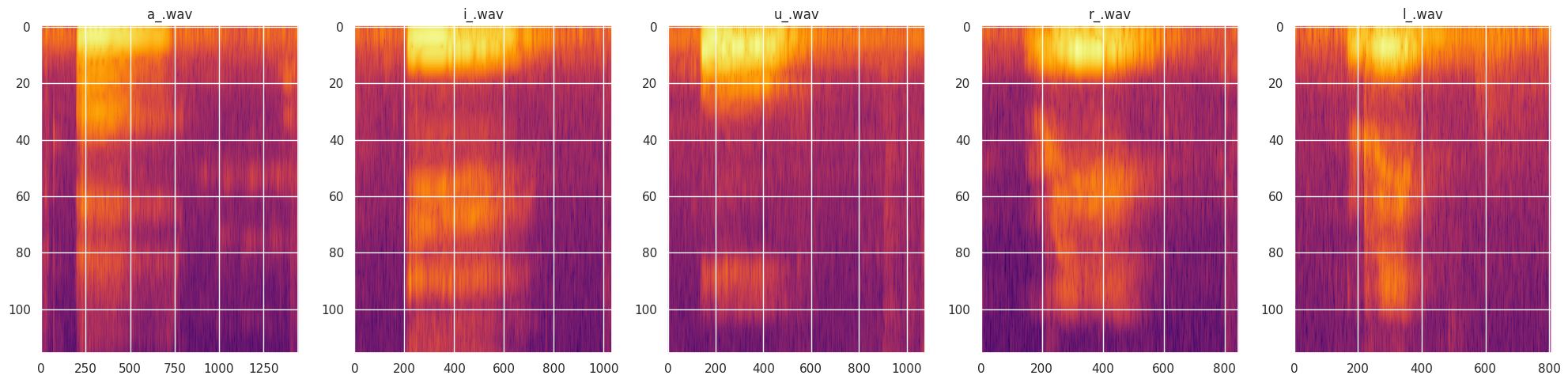
- We can clearly observe the pitch trends in the data in both the cases.
Key Features
- Parselmouth Integration: Direct Python access to Praat algorithms
- Acoustic Analysis: Extract intensity, pitch, formants, and spectral properties
- Visualization: Publication-quality plots of acoustic features
- Statistical Analysis: Compute descriptive statistics of speech characteristics
Further Reading
Full Interactive Notebook
For the complete code with additional examples, formant analysis, and advanced techniques, view the interactive notebook:

Kartikay Agrawal
Me n my coffee against the world